Images in Science

Everyone loves a good image, especially when it can easily convey a complex idea.  I currently use POV-Ray ray tracing software to create images for presentations, reports, and journal articles.  The same software can be used to create animations.  This software is appealing to me for a few reasons:  it uses mathematical constructs rather than triangle meshes, it uses code rather than mouse clicks, and the rendered image obeys the physics of light (e.g., lenses magnify what is behind them).  Below are some images created with POV-Ray.  Feel free to use the images, use the code, or modify the code for your own use.  Best practices suggest that you should acknowledge the source of these images or code, but I am not going to hunt you down if you don’t.

Three Dimensional Data Plots

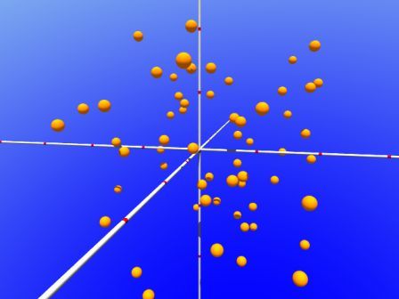Some data are best visualized in three dimensions.  This image shows a dataset of 60 points with x, y, and z coordinates.  One way to generate three dimensional plots is to import the data into POV-Ray, a free and open-source rendering program.  The code below generates these random points and plots them in a coordinate space.  Because everything you see is driven by the code you write, it is completely customizable—If you can imagine it, it can be coded.  You can also create animations of data to show change over time, or to fly through your data.  To animate, you simply tie the position of the objects or the camera/viewer to the clock time.  For example, if you want the camera location to spin in a circle around the data cloud, simply make the x and z coordinates sine and cosine functions of the clock as it ticks from 0 to 1 in any increment you specify.  The code below can be dropped into a new script in POV-Ray to generate the image above.  I may turn this into a series on different ways to visualize data.  If you are interested in seeing the code modified to achieve some effect, let me know.

//  #####  3D Data Plots – Basic  #####
//  #####      JDH, Oct 2015      #####

#include “colors.inc”

//  #####  The Environment  #####
//  #############################
global_settings {ambient_light <1,1,1>*1.4}

light_source{<16, 150, -80> color rgb<1,1,1>*2}
camera{location<1, 1, -5> look_at<0,0,0>}
sky_sphere {pigment {gradient y
color_map {
[0.0 color Blue]
[1.0 color Turquoise] }
rotate x*-40
}}

//  #####  The Coordinate Axes  #####
//  #################################
#declare axis=cylinder{<-6,0,0>, <6,0,0>,0.02
pigment{gradient x color_map{
[0.0 color White]
[0.95 color White]
[0.95 color Red]
[1.0 color Red]
}}
finish{ambient 0.2}
};
object{axis}
object{axis rotate z*90}
object{axis rotate y*90}

//  #####  The Data  #####
//  ######################
#declare dpt = sphere{<0,0,0>, 0.08
pigment{color Orange}
finish{ambient 0.4}
}
#declare myrand = seed(1178);
#declare myloop = 1;
#while(myloop < 61)
#declare myx=(4*rand(myrand))-2;
#declare myy=4*rand(myrand)-2;
#declare myz=4*rand(myrand)-2;
object{dpt translate<myx, myy, myz>}
#declare myloop = myloop + 1;
#end