Dispersal models are useful in research to examine how changing parameters alter how animals may move.  As with other models, they are stripped-down versions of reality in nature that can help us ask better questions, but are not used to test hypotheses.  Just for fun, I decided to start a scratch built dispersal model from the ground up.  The image here is the output from this model.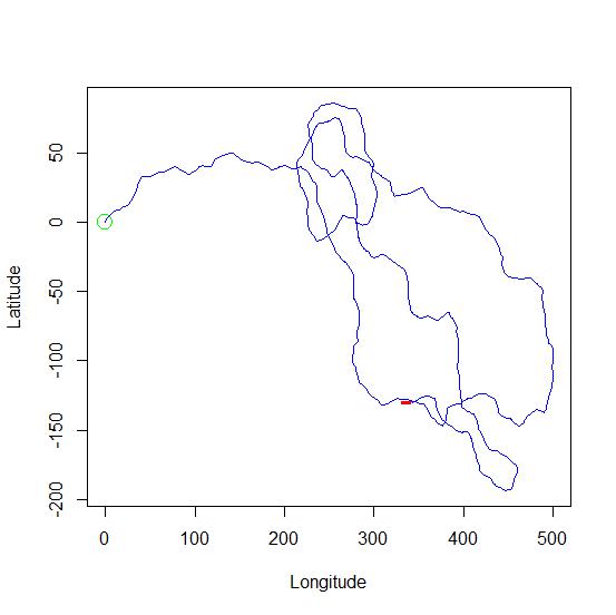 

A single disperser starts at the origin [0,0].  The first movement step is determined by making a random draw from an exponential distribution for the distance moved and a random draw from a normal distribution (mean=0, standard deviation=1/4) for the turning angle in radians, which in the remaining steps will be relative to the last movement.  The resulting new location is stored in a data.frame (a matrix-like object in R), and the step is looped some arbitrary number of times, 1000 steps in this case.

Each path will be different; the probability of returning the same path is infinitesimally small—but that is a post for another day.  However, just as the third theorem of psychohistory states, the overall behavior of the resulting displacement probabilities becomes predictable en mass if many, many, runs are averaged.  I know, the Foundation series is fiction, but I like the analogy.  You cannot use a dispersal model to predict where a specific animal will move, but you may be able to predict how millions will move on average.  With this requirement of many runs necessary to predict the mean movement of a population with millions of animals (or >75 Billion humans in Asimov’s fiction) is this still useful?  Who would be modeling movement of this many animals?  Well, entomologists for one group.  However, with this many motes being simulated, and that movement becoming predictable, we can start to model the spread using something that becomes relatively simpler as the number of motes increases: reaction—diffusion equations.  For now, I am going to continue developing additional uses for this individual-based dispersal model.

The code below is the very beginning of my very simple dispersal model.  The first half is the actual model; most of the code is my clumsy attempt to make it easy to plot.  I will build on this in future posts as I make more progress with it.  Note that the code is very inelegant to show details and to keep things based upon “first principles.”  There are more concise methods, and I would not use these methods in a demanding modeling exercise, but I think understanding the nuts and bolts from the ground up is the best way to do, well, anything.  If you have never opened the hood of a car, then don’t drive a car into the desert alone.  If you have never programmed a dispersal model, don’t try to present the results of a canned dispersal program.  Both of these stories can have bad endings.

posit <- data.frame(nrows=1000, ncol=2)          ##  Create an empty data.frame.
posit[1,1:2] <- c(0,0)                           ##  Start at the origin.
set.seed(4242)                                   ##  Set a random seed.

#########  Calculations  ##########
a.turn <- rnorm(n=1, mean=0, sd=1/4)             ##  Random draw from normal distr.
for(i in 2:1000){                                ##  Open loop.
   a.dist <- rexp(n=1, rate=0.5)                 ##  Random distance from expont'l.
   posit[i,] <- c(posit[i-1,1]+a.dist*(sin(a.turn)),
      posit[i-1,2]+a.dist*(cos(a.turn)))         ##  Update position, a.turn in radians.
   a.turn <- a.turn + rnorm(n=1, mean=0, sd=1/4) ##  Generate next turn angle.
           }                                     ##  End loop. Calcs done!

#########  Rearrange Data for Easier Plotting  ##########
##  To make plotting easier create start & stop coords of each step in same row.
posit.plot <- data.frame(nextx=NA, nexty=NA, long=posit[,1], lat=posit[,2])
posit.plot[1,1:2] <- c(0,0)
for(p in 2:1000){
   posit.plot[p,1:2] <- posit.plot[p-1,3:4]
   }                                              ##  Same data, easier to plot.

##########  The Plot  ##########
plot(posit[,1], posit[,2], xlab="Longitude", ylab="Latitude", type="n")
   segments(posit.plot[,1],posit.plot[,2], posit.plot[,3],posit.plot[,4], col="blue")                 ##  Line segments between sequential positions.
   points(0,0, pch=1, cex=2, col="green")         ##  Power up symbol at start.
   points(posit[1000,1],posit[1000,2], pch="-", cex=2, col="red")    ## End pt.