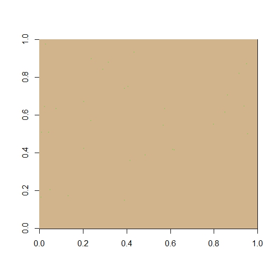
I wished to generate a random landscape map of habitat and non-habitat. This will be the arena for the next development in the correlated random walk dispersal model of last month. The landscape generated has large blocks of habitat, i.e., the cell value of habitat or non-habitat is not randomly determined for each cell which would have led to a predictably random pattern not reminiscent of real landscapes. The code I came up with takes a few input values and generates the required landscape map of habitat.

The first input value determines how large the square landscape should be. I used 1000 to generate a landscape that is 1000 cells on a side, or one million cells. Further down in the code I turned translated this raster both south and west by half of the size value so that the center is at coordinates (0,0). I then turned it into a raster layer with a cell size of 1 m x 1 m.  The units do not matter for this exercise, only the numerals.

The next input value determines the initial probability of each cell being habitat. Each cell will be assigned a value drawn from a binomial distribution with the designated probability of being habitat. These cells will form the “seeds” upon which our habitat patches will grow. In the example I used a probability of 0.0002 so that 1 in 5,000 cells will initially be habitat (green) and the rest will be non-habitat (tan).

The isolated habitat cells do not show up here well because the jpg image format is smoothing over them. They are there, approximately 200 of them. To expand the few habitat cells into larger contiguous patches of habitat I employed a shortcut by using a moving window to expand them. I created a second matrix that is essentially a diamond shape of value=1 within a 5 x 5 matrix of value=0. For example, the top row was [1,] = 0,0,1,0,0, and the second row was [2,]=0,1,1,1,0. This matrix was the window that I slide across the 1000 x 1000 cell landscape. The window moved across the entire landscape one row and one lateral cell at time. At each stop, it examined the landscape values under the window and applied the function=maximum, weighted according to the ones and zeros in the window matrix. In other words, it found the maximum value of the landscape under the value=one cells. This value was then assigned to the cell in the landscape matrix that fell directly underneath the window matrix. The window then shifted one cell over and repeated the process. The end result, is that the original “seed’ cells grew as the window passed over them.

The third value is the expansion value. Each time the moving window algorithm is applied the habitats in the landscape raster grow. The expansion value determines how many times the moving window is applied iteratively. The figure here shows the original sample landscape passed through the moving window expansion 17 times. This raster is now ready for electronic critters to start scampering across. The code is below.

library(raster)

ls.size <- 1000					## Set ls size, side dimension.
exp.num <- 17					## Set number of expansions.
hab.seed <- 0.0002				## Set Pr(hab) in initial binomial.
set.seed(542)
my.ls.val <- matrix(data=rbinom(n=ls.size*ls.size, size=1, prob=0.0002),
	nrow=ls.size, ncol=ls.size)
image(my.ls.val, col=c("tan", "green"))

my.ls <- raster(ncol=ls.size, nrow=ls.size, xmn=-1*(ls.size/2),
	xmx=ls.size/2, ymn=-1*(ls.size/2), ymx=ls.size/2, res=1)
projection(my.ls) <- "+proj=utm +zone=16 +datum=NAD83"
values(my.ls) <- my.ls.val

nbrhood.n <- matrix(data=c(0,0,1,0,0,0,1,1,1,0,1,1,1,1,1,0,1,1,1,0,0,0,
	1,0,0), nrow=5, ncol=5)
nbrhood <- nbrhood.n/sum(nbrhood.n)

for(i in 2:exp.num){
	my.new.ls <- focal(my.ls, w=nbrhood, fun=max, pad=2, padValue=0)
	my.ls <- my.new.ls
	}

image(my.ls, col=c("tan", "green"))